출처 : http://the-paper-trail.org/blog/columnar-storage/
Columnar Storage
You’re going to hear a lot about columnar storage formats in the next few months, as a variety of distributed execution engines are beginning to consider them for their IO efficiency, and the optimisations that they open up for query execution. In this post, I’ll explain why we care so much about IO efficiency and show how columnar storage – which is a simple idea – can drastically improve performance for certain workloads.
Caveat: This is a personal, general research summary post, and as usual doesn’t neccessarily reflect our thinking at Cloudera about columnar storage.
Disks are still the major bottleneck in query execution over large datasets. Even a machine with twelve disks running in parallel (for an aggregate bandwidth of north of 1GB/s) can’t keep all the cores busy; running a query against memory-cached data can get tens of GB/s of throughput. IO bandwidth matters. Therefore, the best thing an engineer can do to improve the performance of disk-based query engines (like RDBMs and Impala) usually is to improve the performance of reading bytes from disk. This can mean decreasing the latency (for small queries where the time to find the data to read might dominate), but most usually this means improving the effective throughput of reads from disk.
The traditional way to improve disk bandwidth has been to wait, and allow disks to get faster. However, disks are not getting faster very quickly (having settled at roughly 100 MB/s, with ~12 disks per server), and SSDs can’t yet achieve the storage density to be directly competitive with HDDs on a per-server basis.
The other way to improve disk performance is to maximise the ratio of ‘useful’ bytes read to total bytes read. The idea is not to read more data than is absolutely necessary to serve a query, so the useful bandwidth realised is increased without actually improving the performance of the IO subsystem. Enter columnar storage, a principle for file format design that aims to do exactly that for query engines that deal with record-based data.
Columns vs. Rows
Traditional database file format store data in rows, where each row is comprised of a contiguous collection of column values. On disk, that looks roughly like the following:

This row-major layout usually has a header for each row that describes, for example, which columns in the row are NULL. Each column value is then stored contiguously after the header, followed by another row with its own header, and so on.
Both HDDs and SSDs are at their most efficient when reading data sequentially from disk (for HDDs the benefits are particularly pronounced). In fact, even a read of a few bytes usually brings in an entire block of 4096 bytes from disk, because it is effectively the same cost to read (and the operating system usually deals with data in 4k page-sized chunks). For row-major formats it’s therefore most efficient to read entire rows at a time.
Queries that do full table-scans – i.e. those that don’t take advantage of any kind of indexing and need to visit every row – are common in analytical workloads; with row-major formats a full scan of a table will read every single byte of the table from disk. For certain queries, this is appropriate. Trivially, SELECT * FROM table requires returning every single column of every single row in the table, and so the IO costs for executing that query on a row-major format are a single-seek and a single large contiguous read (although that is likely to be broken up for pipelining purposes). The read is unavoidable, as is the single seek; therefore row-major formats allow for optimal IO usage. More generally, SELECT <col_set> FROM table WHERE <predicate_set> will be relatively efficient for row-major formats if either a) evaluating the predicate_set requires reading a large subset of the set of columns or b) col_set is a large subset of the set of columns (i.e. the projectivity is high) and the set of rows returned by the evaluation of the predicates over the table is a large proportion of the total set of rows (i.e. the selectivity is high). More simply, a query is going to be efficient if it requires reading most of the columns of most of the rows. In these cases, row-major formats allow the query execution engine to achieve good IO efficiency.
However, there is a general consensus that these SELECT * kinds of queries are not representative of typical analytical workloads; instead either a large number of columns are not projected, or they are projected only for a small subset of rows where only a few columns are required to decide which rows to return. Coupled with a general trend towards very wide tables with high column counts, the total number of bytes that are required to satisfy a query are often a relatively small fraction of the size on disk of the target table. In these cases, row-major formats often are quite wasteful in the amount of IO they require to execute a query.
Instead of a format that makes it efficient to read entire rows, it’s advantageous for analytical workloads to make it efficient to read entire columns at once. Based on our understanding of what makes disks efficient, we can see that the obvious approach is to store columns values densely and contiguously on disk. This is the basic idea behind columnar file formats. The following diagram shows what this looks like on disk:

A row is split across several column blocks, which may even be separate files on disk. Reading an entire column now requires a single seek plus a large contiguous read, but the read length is much less than for extracting a single column from a row-major format. In this figure we have organised the columns so that they are all ordered in the same way; later we’ll see how we can relax that restriction and use different orderings to make different queries more efficient.
Query Execution
The diagram below shows what a simple query plan for SELECT col_b FROM table WHERE col_a > 5 might look like for a query engine reading from a traditional row-major file format. A scan node reads every row in turn from disk, and streams the rows to a predicate evaluation node, which looks at the value of col_a in each row. Those rows that pass the predicate are sent to a projection node which constructs result tuples containing col_b.

Compare that to the query plan below, for a query engine reading from columnar storage. Each column referenced in the query is read independently. The predicate is evaluated over col_a to produce a list of matching row IDs. col_b is then scanned with respect to that list of IDs, and each matching value is returned as a query result. This query plan performs two IO seeks (to find the beginning of both column files), instead of one, and issues two consecutive reads rather than one large read. The pattern of using IDs for each column value is very common to make reconstructing rows easier; usually columns are all sorted on the same key so the Nth value of col_a belongs to the same row as the Nth value of col_b.

The extra IO cost for the row-format query is therefore the time it takes to read all those extra columns. Let’s assume the table is 10 columns wide, ten million rows long and each value is 4 bytes, which are all conservative estimates. Then there is an extra 8 * 1M * 4 bytes, or 32MB of extra data read, which is ~3.20s on a query that would likely otherwise take 800ms; an overhead of 300%. When disks are less performant, or column widths wider, the effect becomes exaggerated.
This, then, is the basic idea of columnar storage: we recognise that analytical workloads rarely require full scans of all table data, but do often require full scans of a small subset of the columns, and so we arrange to make column scans cheap at the expense of extra cost reading individual rows.
The Cost of Columnar
Is this a free lunch? Should every analytical database go out and change every file format to be column-major? Obviously the story is more complicated than that. There are some query archetypes that suffer when data is stored in a columnar format.
The obvious drawback is that it is expensive to reassemble a row, since the separate values that comprise it are spread far across the disk. Every column included in a projection implies an extra disk seek, and this can add up when the projectivity of a query is high. Therefore, for highly projective queries, row-major formats can be more efficient (and therefore columnar formats are not strictly better than row-major storage even from a pure IO perspective).
There are more subtle repurcussions of each row being scattered across the disk. When a row-major format is read into memory, and ultimately into CPU cache, it is in a format that permits cheap reference to multiple columns at a time. Row-major formats have good in-memory spatial locality, and there are common operations that benefit enormously from this.
For example, a query that selects the sum of two columns can sometimes be executed (once the data is in memory) faster on row-major formats, since the columns are almost always in the same cache line for each row. Columnar representations are less well suited; each column must be brought into memory at the same time and moved through in lockstep (yet this is still not cache efficient if each column is ordered differently), or the initial column must be scanned, each value buffered and then the second column scanned separately to complete the half-finished output tuple.
The same general problem arises when preparing each tuple to write out as a result of (non-aggregating) query. Selecting several columns at once requires ‘row reconstruction’ at some point in the query lifecycle. Deciding when to do this is a complicated process, and (as we shall see) the literature has not yet developed a good rule of thumb. Many databases are row-major internally, and therefore a columnar format is transposed into a row-major one relatively early in the scanning process. As described above, this can require buffering half-constructed tuples in memory. For this reason, columnar formats are often partiioned into ‘row-groups’; each column chunk N contains rows (K*N) to ((K+1) * N). This reduces the amount of buffering required, at the cost of a few more disk seeks.
Further Aspects of Columnar Storage
Fully column-oriented execution engines
Relevant papers:
C-Store: A Column-oriented DBMS
The Vertica Analytic Database: C-Store 7 Years Later
Materialization Strategies in a Column-Oriented DBMS
Performance Tradeoffs in Read-Optimized Databases
Column-Stores vs. Row-Stores: How Different Are They Really?
In this post, I’ve talked mostly about the benefits of columnar storage for scans – query operators that read data from disk, but whose ultimate output is a batch of rows for the rest of the query plan to operate on. In fact, columnar data can be integrated into pretty much every operator in a query execution engine. C-Store, the research project precursor to Vertica, explored a lot of the consequences of keeping data in columns until later on in the query plan. Eventually, of course, the columns have to be converted to rows, since the user expects a result in row-major format. The choice of when to perform this conversion is called late or early materialisation; viewed this way column-stores and row-stores can be considered two points on a spectrum of early to late materialisation strategies. Materialisation is studied in detail in the materialisation strategies paper above. Their conclusions are that the correct time to construct a tuple depends on the query plan (two broad patterns are considered: pipelining and parallel scans) and the query selectivity. Unfortunately, supporting both strategies would involve significant implementation cost – each operator would have to support two interfaces, and two parallel execution engines would effectively be frankensteined together. In general, late materialisation can lead to significant advantages: for example, by delaying the cost of reconstructing a tuple, it can be avoided if the tuple is ultimately filtered out by a predicate.
The difference between row-based and columnar execution engines is studied in the Performance Tradeoffs… and Column-Stores vs. Row-Stores… papers. The former takes a detailed look at when each strategy is superior – coming out in favour mostly of column-stores, but only with simple queries and basic query plans. The latter tries to implement common column-store optimisations in a traditional row-store, without changing the code. This means a number of increasingly brittle hacks to emulate columnar storage.
Compression
Relevant papers:
Integrating Compression and Execution on Column-Oriented Database Systems
A column of values drawn from the same set (like item price, say) is likely to be highly amenable to compression since the values contained are similar, and often identical. Compressing a column has at least two significant advantages on IO cost: less space is required on disk, and less IO required to bring a column into memory (at the cost of some CPU to decompress which is usually going spare). Some compression formats – for example run-length encoding – allow execution engines to operate on the compressed data directly, filtering large chunks at a time without first decompressing them. This is another advantage of late materialisation – by keeping the data compressed until late in the query plan, these optimisations become available to many operators, not just the scan.
Hybrid approaches
Relevant papers:
Weaving Relations for Cache Performance
Since neither row-major nor column-major is strictly superior on every workload, it’s natural that some research has been done into hybrid approaches that can achieve the best of both worlds. The most commonly known approach is PAX – Partition Attributes Across – which splits the table into page-sized groups of rows, and inside those groups formats the rows in column-major order. This is the same approach as the row-groups used to prevent excessive buffering described earlier, but this is not the aim of PAX; with PAX the original intention was to make CPU processing more efficient by having individual columns available contiguously to perform filtering, but also to have all the columns for a particular row nearby inside a group to make tuple reconstruction cheaper. The result of this approach is that IO costs don’t go down (because each row-group is only a page long, and is therefore read in its entirety), but reconstruction and filtering is cheaper than for true columnar formats.
'빅데이터' 카테고리의 다른 글
| Apache Drill vs. Apache Spark: What’s The Right Tool for the Job? (0) | 2016.07.11 |
|---|---|
| Hello, TensorFlow! (0) | 2016.07.08 |
| 분산 로그 수집기 Fluentd 소개 (0) | 2016.06.14 |
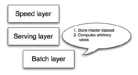
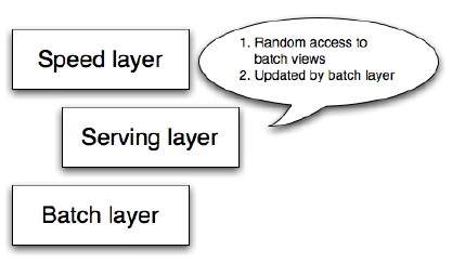
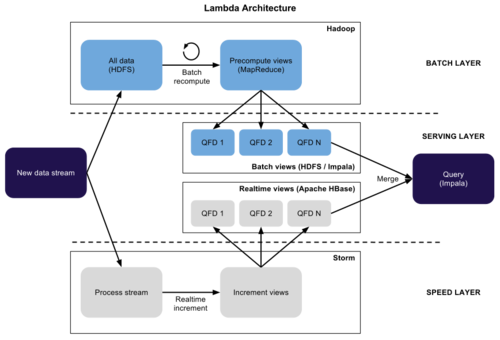
| 람다 아키텍처(Lambda Architecture) (0) | 2016.05.18 |
| Lambda Architecture (0) | 2016.05.18 |


 Samza’s solution for everything is just push it out to Kafka and problem solved, and it also works in the context of state management. Samza has real stateful operators so any task can hold a state and the state’s change log is pushed to Kafka. If needed state can be easily recreated from Kafka’s topic. To make it a little bit faster Samza allows us to plug-in key-value stores as a local storage so it doesn’t have to go to the Kafka all the time. The concept is illustrated on the picture below. Unfortunately, Samza provides at-least one semantics only, and it hurts a lot, but the implementation of exactly once delivery is planned.
  Flink provides stageful operators conceptually similar to Samza. When working with Flink, we can use two different types of states. First one is local or task state, it is a current state of particular operator instance only and these guys don’t interact between each other. Then we have partitioned, or if you want key state, which maintains state of whole partitions. And of course, Flink provides exactly-once semantics. In the picture below you can see outline of Flink’s long running operator with 3 local states.


